HoloBright will present some research blogs on optical interferometric measurement system. We will frequently update the blog and hope it is useful to researchers and students who are working in opto-mechanics area.
1, Interferometric dynamic measurement: Techniques based on high-speed imaging or a single photodetector
ABSTRACT
In recent years, optical interferometry-based techniques have been widely used to perform noncontact measurement of dynamic deformation in different industrial areas. In these applications, various physical quantities need to be measured in any instant and the Nyquist sampling theorem has to be satisfied along the time axis on each measurement point. Two types of techniques were develop for such measurements: one is based on high-speed-cameras and the other uses a single photodetector. The limitation of the measurement range along the time axis in camera-based technology is mainly due to the low capturing rate; while the photodetector-based technology can only do the measurement on a single point. In this paper, several aspects of these two technologies are discussed. For the camera-based interferometry, the discussion includes the introduction of the carrier, the processing of the recorded images, the phase extraction algorithms in various domains, and how to increase the temporal measurement range by using multi-wavelength techniques. For the detector-based interferometry, the discussion mainly focuses on the single-point and multi-point laser Doppler vibrometers and their applications for measurement under extreme conditions. The results show the effort done by researchers for the improvement of the measurement capabilities using interferometry-based techniques to cover the requirements needed for the industrial applications.
Keywords: Dynamic measurement, interferometry, carrier, phase retrieval, laser Doppler vibrometry.
1. Introduction
In the last several decades, the drive for higher performance and reliability of devices, structures, and processes in engineering has placed stringent demands on the methods used in their development, and measurement. Optical metrology is a major and inseparable part of the measurement methods. The field of optical metrology is arguably more than one century old. However, major advances have resulted from the invention of laser only about fifty years ago. This new light source opened a realm of new techniques to both the physicist and the engineer. With the advent of the laser, coherent optics has been brought into measurement techniques of various areas. Optical interferometry [1] is a well-known technique to measure the path-length change of laser light caused by deformation, or movement, or unevenness of an object. Generally, there are two types of techniques: one is based on two-dimensional sensor like CCD or CMOS camera and the other is based on single-pixel photodetector.
1.1 Interferometric dynamic measurement (IDM)
The typical camera-based interferometry include different methods, such as: photoelasticity [2], moiré interferometry [3], Electronic Speckle Pattern Interferometry (ESPI) [4], Shearography [5], digital holography [6], white-light interferometry [7] etc. Generally, they are non-contacting and whole-field techniques providing results in the form of fringe patterns that represent different physical quantities, such as distance, in-plane or out-of-plane displacements, strain, stresses or refractive-index. Although a fringe pattern representing distance, deformation or distortion is readily obtained, expert interpretation is necessary to convert these fringes into desired information. For the accurate mapping of these physical quantities various fringe processing algorithms, notably the Fourier transform [8] and phase shifting [9], have been used. Due to the limited capturing rate of the camera and the long processing time for fringe pattern, initially these interferometers were mainly used for quasi static measurements. For high-frequency periodical vibration measurement, the camera-based interferometry is applied to determine vibration modes of objects. Time-average methods, based on digital holography [10], ESPI [11], DSSI [12], or Moiré [13] directly acquire a spatially dense, full-field, real-time image of the mode shape, while other techniques require the reconstruction of the mode shape from single point measurements. Methods using stroboscopic light sources [14] allow to “fix” the steady-state vibration and can be applied in principle for the measurement of non-sinusoidal vibrations, but the movement should be periodical. In addition, if low-speed CCDs are used, the time for acquiring the interferograms may be quite long and this make the technique poorly suited to be used in an industrial environment.
In many cases, high-resolution three-dimensional (3-D) dynamic displacement or surface profiling can give useful information about the dynamic response of a mechanical structure. However, it is difficult to achieve this with the above-mentioned techniques. The use of a twin-cavity double-pulse laser interferometry [15] has been reported as an alternative to obtain transient deformations. However, this technique has a fatal limitation, since to obtain the evolution of the transient deformation, an experiment must be repeated many times with a different interval of two pulses. This means that non-repeatable events cannot be studied in detail. Due to the rapid development of high-speed digital recording devices, it is possible to record interferograms with rates exceeding 100,000 frame/s. In order to measure various physical quantities at any instant, high-speed camera is adopted in various interferometric techniques to satisfy the Nyquist sampling theorem along time axis. This leads to a series of interferometric dynamic measurement techniques based on high-speed imaging.
On the other hand, single-pixel detector-based interferometry has already been successfully applied for dynamic measurement. Laser Doppler vibrometry [16] and laser Doppler velocimetry [17] are two similar techniques, the former one is for the measurement of out-of-plane displacement or velocity and the latter one is for in-plane displacement or velocity measurement. Compared to a full-field measurement based on high-speed camera, detector based interferometry can only offer a point-wise measurement, but with large measurement velocity range. For the extraction of the Doppler frequency shift, different interferometric solutions can be used. The heterodyne Mach-Zehnder and the homodyne Michelson interferometers are two typical configurations. In order to measure the vibration at different points, Laser Doppler vibrometers are equipped with a video camera and a scanning system. These scanning laser Doppler vibrometers (SLDV) give the possibility of moving the measurement point rapidly and precisely on the testing surface, allowing the analysis of large surface with high spatial resolution [18].
1.2 Current status of IDM
Figure 1 shows that the camera-based technique has very high spatial resolution but its temporal resolution is low compared with the requirement of real applications. Even a 100k frame/s capturing rate sometimes cannot satisfy the Nyquist sampling theorem, as for every measurement point, the phase change of any two adjacent images should be less than π. In addition, a high power laser is needed for the illumination and the cost of high-speed camera also limits the applications in industrial areas. On the contrary, detector-based laser Doppler techniques have enough sampling rate along the time axis, but only one measurement point in spatial domain. A scanning device is usually used to perform 2-D measurements. This method assumes that the measurement conditions remain invariant while sequential measurements are performed. Hence, it is only suitable to measure steady-state or well-characterized vibrations. However, most engineering applications do not satisfy these requirements. Transients, including impact or coupled vibrations, are commonly observed in real applications and scanning LDVs impractical to generate a vibration image in these cases.

Fig. 1 The current status of camera-based and detector-based interferometry
In this paper, some new measurement and processing technologies based on high-speed imaging and detector are reviewed. Several issues of the camera-based IDM are discussed, these include the carrier and processing domain, phase extraction technique and how to increase the measurement range by using the multi-wavelength method. A detector-based IDM technique using a multi-point laser Doppler vibrometer (LDV) based on a spatially-encoded technology is described. Some applications under extreme conditions are presented and the results show the trend of IDM to meet the requirements necessary for industrial applications with sufficient temporal and spatial sampling points.
2. High-speed-imaging-based IDM
In the high-speed-imaging-based interferometric dynamic measurement technique (IDM), the signal obtained is a sequence of interferograms recorded at time t (see Fig. 2), that can be written as:
![]() (1)
(1)
Where and are the intensity bias and the modulation factor, respectively. These two items are both slowly carrying functions along the time axis. is a phase variation due to a vibration or a continuous displacement. is the initial phase value of each pixel. The purpose of the imaging-based IDM is to extract the phase from a 3-D matrix as expressed in Eq. (1).
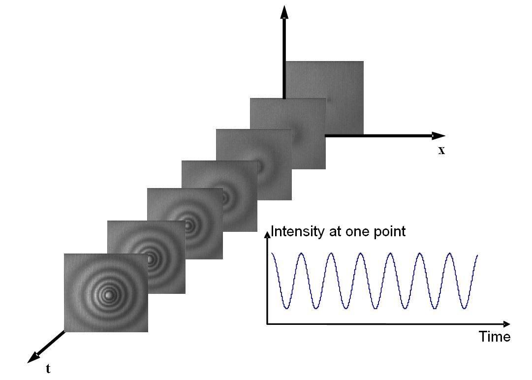
Fig.2 Schematic layout of the high-speed-imaging-based IDM
2.1 Phase extraction techniques
There are quite a lot of phase extraction techniques for interferometric fringe patterns and these are classified into three categories: phase-shifting methods, transform-based methods and others.
2.1.1 Phase-shifting techniques
The phase-shifting techniques can be classified into temporal and spatial phase shifting. In the temporal phase shifting technique, at least three phase-shifted fringe patterns or specklegrams are collected. In order to keep the phase nearly unchanged during the phase shifting, a fast phase shifter and a high capturing rate are necessary. In 1996, De Lega and Jacquot [19] proposed the object-induced temporal phase changes where a piezoelectric transducer (PZT) with the driven frequency of 80 Hz was used to produce a phase shift between two consecutive frames. In 1999, Huntley et al. [20] developed a phase shifting speckle interferometer operated at 1k Hz capturing rate using a high-speed camera. A Pockels cell producing a phase shift of between two consecutive frames was used and the system was synchronized with the camera. In 2003, Kaufmann [21] used a similar system to monitor the out-of-plane deformation of a plate with flaw. In these techniques, temporal phase unwrapping [22] was applied. Hence, the measurement errors were also accumulated. In 2002, Kao et al. [23] applied the phase shifts to the initial status , but not to other instances . Phase-shifted speckle-correlation fringe patterns can be formed between and . This method is very simple, but suffers from speckle decorrelation. In 2005, the re-referencing rate, i.e., the update rate of the reference frame, was studies [24] to avoid the influence of the speckle decorrelation. Generally, the temporal phase-shifting method is only suitable to measure a slow-varying deformation or profile changing producing a phase variation which is much slower compared with the temporal carrier generating the reference phase shift. .
In the spatial phase-shifting techniques, several phase-shifted fringe patterns are captured in one shot at different locations by either different cameras or on different areas of a camera. Several such systems are described in Refs. [25 -27]. A significant innovation is a camera with a pixelated phase mask that can be combined with different interferometers [28, 29]. This technique converts a 2×2 superpixel into four phase-shifted pixels using micro-polarizers, avoiding the registration of several phase-shifting fringe patterns. Compared to temporal phase-shifting techniques, the measurement range along the time-axis is increased, with the cost of slightly sacrificing the spatial resolution. Similar technique can be found in fringe projection profilometry [30], although this is not considered as an interferometric technique.
2.1.2 Transform-based techniques
Transform-based techniques are the predominant phase extraction methods in the imaging-based IDM. These techniques include Fourier transform [8], Hilbert transform [31], windowed Fourier transform [32], wavelet transform [33] and a combination of Fourier and windowed Fourier transform [34]. Like the phase-shifting techniques, the transform-based phase extraction methods can be applied in the spatial domain, temporal domain, or even spatial-temporal domain. The processing can be one-dimensional (1-D), 2-D or even 3-D. The only requirement is that a carrier has to be introduced along one-axis in the processing domain to avoid the phase ambiguity. Carrier-based 2-D spatial Fourier transform [8] was firstly applied in IDM as it allows to extract the phase distribution from a single carrier fringe pattern. It has been applied to measure the transient phenomena by Moiré interferometry [35] and speckle interferometry. A spatial carrier leads to a fringe pattern with various fringe densities in one image. However, in the speckle interferogram, the fringe density cannot be too high due to the speckle noise and this limits the measurement. In recent years, other transforms such as windowed Fourier transform [32] and wavelet transform [33] have also been used to process the carrier fringe pattern.
After the introduction of the high-speed camera in IDM, a temporal version of the Fourier analysis and other transform-based methods were applied to extract the phase. In this case, a temporal carrier is required. In 1998, Joenathan et al. performed a series of studies on temporal phase evaluation through speckle interferometry for out-of-plane deformation [36], in-plane deformation [37], the derivative of out-of-plane deformation [38], and the shape measurement [39]. The influence of decorrelation, speckle size, and non-linearity of the camera were also discussed [40] and a rotating half-wave plate was proposed to introduce a temporal carrier. In 2002, Kaufmann and Galizzi compared the temporal phase-shifting method with the temporal Fourier transform method [41]. In 1997, De Lega firstly described a temporal wavelet phase extraction algorithm for dynamic measurement [42]. The research was continued by Fu et al. [43, 44] as well as Federico and Kaufmann [45]. The S transform, a similar algorithm to wavelet transform, has also been used for temporal phase evaluation [46]. Another technique is the windowed Fourier transform (WFT). In 2003 Ruiz et al. elegantly linked a temporal phase-shifting algorithm to the temporal windowed Fourier transform, and showed that the WFT provided better performance [47]. In 2006, Qian et al. applied a 3-D WFT to process a sequence of fringe pattern from speckle interferometry [48]. In 2007, Fu et al. applied the WFT to digital holography for vibration measurement and demonstrated its superior performance over the Fourier transform [49]. In the same year, they proposed a combination of two transforms, namely, the temporal Fourier transform and the spatial windowed Fourier transform, and showed that this combination performed better than either single transform [34].
2.1.3 Miscellaneous algorithms
Another simple but effective temporal phase extraction algorithm, time sequence analysis, was proposed by Li et al. in 2001-2004 [50-52]. It includes phase scanning method, sequence pulse counting method, and matched correlation sequence analysis. Theses methods retrieve the phase from the variation of the gray values. The significant advantage of the time sequence analysis algorithm is its simple and efficient. The drawback is that it cannot be applied to a very noisy signal as the accuracy of the methods relies on the correct identification of the fluctuations of the interference intensity in each cycle. Li also applied this algorithm to speckle fringe patterns but the method is more suitable for low noise patterns obtained by incoherent methods such as fringe projection and shadow moiré. Furthermore, it needs enough sampling points in one cycle of gray value variation. Li mentioned at least 6 sampling points, but from the experiments it was found that 10 to 16 sampling points per cycle produce the best results.
In recent years, some algorithms for the extraction phase values from one fringe pattern without spatial carrier were reported [53-57]. However, these algorithms are based on some assumptions and they may be working on some fringe patterns but fail on others. Hence, adding a carrier frequency is still the most reliable and effective method.
2.2 Carrier and processing domain
For the interferometric dynamic measurement, the carrier can be introduced either in the spatial domain (along x- or y- axis) or in the temporal domain (along the t-axis). Table 1 shows the comparison of spatial and temporal carrier-based techniques. In the spatial-carrier-based technique, the quality of the retrieved phase map is affected by several factors, such as speckle noise, non-uniform reflectivity, irregular shape of the surface, etc. Figure 1 gives an example of the effect of irregular shape of surface in the fringe projection technique. Although fringe projection is not an interferometric method, the problem involved in the fringe processing is the same as in interferometry. In fringe projection the carrier already exists in the spatial domain. However, the result of the spatial processing will be seriously affected by a non-uniform reflectivity of the surface or a height step on the surface. Zero-padding is also needed for an irregular shape and this will also generate large error at the edge. Figure 3(a) shows a fringe pattern projected on a cantilever beam with irregular shape. Figures 3(b) and 3(c) show a wrapped phase map after 2-D Fourier transform and the phase distribution after unwrapping and removal of the carrier. The phase distortion close to the edge is due to the zero-padding. The results obtained by WFT and CWT are worse due to their lower resolutions in the spatial and frequency domains. This example shows that spatial processing may not be a good choice in some cases.
Table 1. Comparison of spatial-carrier and temporal-carrier-based techniques in interferometry
| Factors | Spatial-carrier-based technology | Temporal-carrier-based technology |
| Processing domain | x- & y- axis | t- axis |
| Dimension | 2-D | 1-D |
| Reflectivity | Affected by non-uniform reflectivity | Not affected |
| Height step | Affected by height step of test objects | Not affected |
| Shape | Affected by irregular shape of surface | Not affected |
| Retrieved phase map quality | Poor, affected by speckle noise when laser is used | Much better than spatial carrier as the process is 1-D along time axis. |
| Measurement range in temporal domain | Determined by Nyquist sampling theorem | Affected by temporal carrier, much less measurement range than spatial carrier |

(a) (b) (c)
Fig. 3 (a) Typical fringe pattern on a cantilever beam with irregular shape; (b) wrapped phase obtained by 2D spatial transform; (c) phase distribution after unwrapping and removal of the carrier.
Figure 4 shows a comparison of spatial and temporal carriers in digital shearography [58]. In this technique, the phase change represents the deflection derivative. Figure 4(a) shows a shearographic fringe pattern with spatial carrier on a fully-clamped circular plate with central-point loading where the nearly straight parallel carrier modulate the shearography fringes. The density of the carrier fringes should be high enough to enable the unambiguous determination of the fringe orders. A two-dimensional Fourier transform is then applied to extract the phase from one fringe pattern. The quality of the phase map depends on the proper selection of the band-pass filtering window. Figure 4(b) shows the best result obtained. However, the noise effect is still obvious on the phase map. Figure 4(c) shows the unwrapped phase map after removal of the carrier. Figure 4(d) shows a typical shearography fringe pattern obtained from a dynamic measurement when a temporal carrier is introduced. The fringe density is much higher in this case. The wrapped phase map after temporal analysis and unwrapping are shown in Figs. 4(e) and 4(f), respectively. We may see that good results can be obtained even when the fringes are dense.

Fig. 4 (a) Typical shearography fringe pattern, (b) wrapped phase map and (c) phase after unwrapping and removal of the spatial carrier; (d) shearography fringe pattern, (e) wrapped phase map and (f) phase after unwrapping when the temporal carrier is applied. [Reprint from Optical Engineering, vol.51 pp083602, 2012]
This example shows that the processing along the time-axis usually gives better results, however, due the capturing rate of camera a carrier in the temporal domain will dramatically reduce the measurement range along the time-axis limiting the applications. Hence, a compromise is necessary between these two techniques. This leads to a trade-off processing in the spatial-temporal domain. The carrier is still in the spatial domain but a 2-D algorithm (FFT or WFT) is applied in the spatial-temporal domain [59]. Figure 5 shows an image-plane digital holographic microscopy setup sensitive to out-of-plane displacements. A spatial carrier is introduced by proper positioning of the fiber tip carrying the reference beam. A sequence of digital holograms is captured during the vibration of cantilever beam excited by a PZT.

Fig.5 Schematic layout of an image-plane digital holographic microscope [Reprint from Applied Optics, vol.48(11), pp1992, 2009]
A 2-D Fourier analysis is applied at each interferogram to obtain a series of 2-D wrapped phase maps. The temporal phase variations along the central-line of the cantilever beam generate a spatio-temporal distribution as shown in Fig. 6(a). Phase unwrapping along the time axis yields a continuous phase map [Fig. 6(b)], from which the instantaneous displacement along the central-line can be calculated. Figure 6(c) shows the displacement of the beam at different time tn. Figure 6(d) shows the displacement variation of two points located on the central line at the positions and . The phase values in Fig. 6(a) are then converted to the exponential values and processed in the spatial-temporal domain by using the windowed Fourier ridge algorithm to extract the instantaneous velocity and acceleration.
2.3 Dual-wavelength technique
In many IDM cases, the frequency of the vibrating object is low and the amplitude large. As the measurement still needs to satisfy Nyquist theorem, the requirement on capturing rate should still be very high. In this case, a longer wavelength can effectively increase the measurement range. Lasers emitting infrared radiation ( e. g. 10. 6 µm CO2 laser) are available but unfortunately for such wavelengths the detectors are very expensive and have limited resolution. Hence, dual and multi-wavelength techniques were introduced to generate a longer synthetic wavelength. Different types of dual-wavelength interferometers have been reported during the past several decades. A typical application of dual-wavelength is the measurement of a surface profile with height steps [60]. The method can also be used with digital holography for surface profiling where the phase at single wavelength can be reconstructed from separately-recorded digital holograms [6, 61]. However, it is not suitable for dynamic measurement since two holograms need to be recorded and reconstructed individually. Here a dual-wavelength interferometer combined with image-plane digital holography is presented to achieve a dynamic measurement on a vibrating object. The object was simultaneously illuminated by two lasers with different wavelengths, and a sequence of digital holograms was captured by a CCD camera [62].

Fig. 6 (a) Wrapped phase map in the spatio-temporal plane; (b) Unwrapped phase map shown the displacement variation in the spatio-temporal plane; (c) Displacement distributions of the cantilever beam at different instants; (d) Displacements of two points on the cantilever beam. [Reprint from Applied Optics, vol.48(11), pp1995, 2009]
A schematic layout of a dual-wavelength image-plane digital holography configuration, sensitive to out-of-plane displacement, is shown in Fig. 7. Two lasers with different wavelengths are used. Light from the first laser is split into an object beam and a reference beam. This object beam illuminates a vibrating specimen with a diffuse surface along a direction ei1. Some light is scattered in the observation direction eo where an image-plane hologram is formed on the CCD sensor, as a result of the interference between the reference beam and the object beam. An aperture is put immediately behind the imaging lens to limit the spatial frequencies of the interference pattern. Similarly a second different laser wavelength is used to generate a second interferogram on the CCD sensor. When these two lasers simultaneously illuminate the object and the detector, the two interferograms will be superimposed on the CCD sensor and one digital hologram containing information about these two interferograms will be obtained.
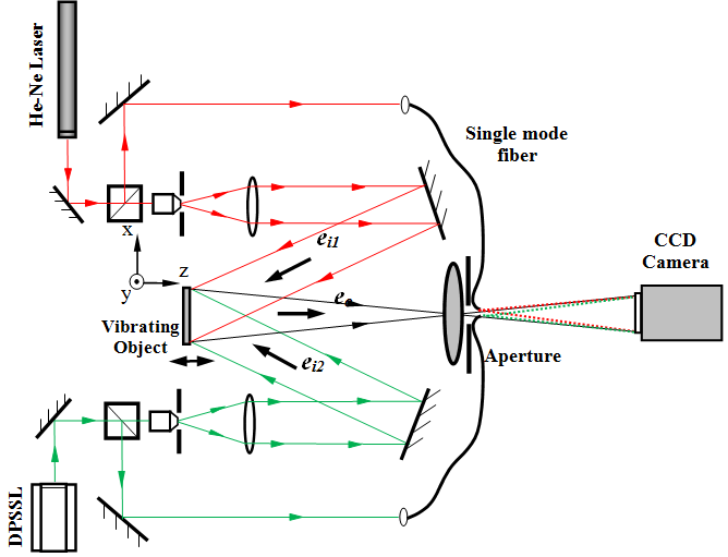
Fig.7 Schematic layout of dual-wavelength image-plane digital holography for dynamic measurement [Reprint from Optics and Lasers in Engineering, vol.47, pp553, 2009]
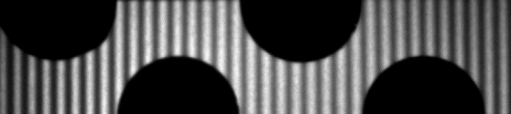
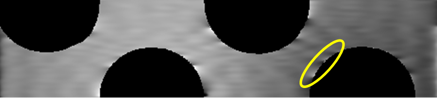
Figure 8(a) shows a typical digital hologram captured by the CCD camera. With a proper selection of the aperture size and a careful adjustment of the two fiber-end positions, it is possible to separate the spectrums of two superimposed holograms in the frequency domain. In our experiment, one hundred and twenty holograms are captured during an eight-second period. Figure 8(b) shows a typical Fourier spectrum of digital holograms captured by the CCD camera. The shadow of the fiber ends can be observed on the spectrums of both digital holograms. When filtering window A is selected, the reconstructed phase difference between the two instants represents the out-of-plane displacement for the wavelength 632.8 nm [Fig. 8(c)]. When filtering window B is selected, the reconstructed phase between the two instants is the result with wavelength of 532nm [Fig. 8(d)]. A slightly difference can be observed between these two wrapped phase maps. At each instant , a new phase distribution is calculated directly by the subtraction of these two wrapped phases:
(2)
where . This phase map is equivalent to a phase distribution of an out-of-plane displacement measurement with a synthetic wavelength , where
(3)

Fig. 8 (a) Typical digital hologram obtained by illumination from two lasers; (b) spectrum of the digital hologram obtained; (c) typical original wrapped phase map with λ1= 633nm; (d) typical original wrapped phase map with λ2= 523nm, and the selected area to process. [Reprint from Optics and Lasers in Engineering, vol.47, pp554, 2009]
Figure 9 shows the phase variation of point C [indicated in Fig. 8(d)] after 1-D temporal phase unwrapping. In our experiment, the synthetic wavelength equals to 3342 nm. In this case, the measurement range in the temporal domain has been increased by 5 times. This is a typical technique to increase the temporal measurement range with the cost of sacrificing some resolution in the spatial domain, which shows the efforts to balance the temporal and spatial resolutions in IDM.
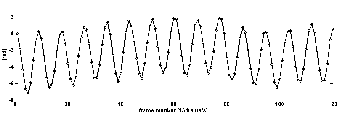
Fig. 9 Phase variation of the point C with the synthetic wavelength of 3342 nm which is proportional to the displacement of the object. [Reprint from Optics and Lasers in Engineering, vol.47, pp556, 2009]
3. Detector-based IDM
Detector-based interferometry is usually used for high temporal resolution point-wise measurements and allows to measure large vibrations amplitudes and frequencies. Two specifications of various single-pixel detectors make the detector-based IDM an effective method for industrial applications: (1) large pixel area; (2) wide frequency response. The detectors size is more than several tens of micrometer, many of them are >0.5 mm with an output bandwidth of 1GHz. Compared to CCD or CMOS cameras, they are more sensitive to low-power laser light. Typical detector-based interferometry includes two similar technologies: laser Doppler vibrometer for out-of-plane displacement or vibration measurement [16], and laser Doppler velocimeter for in-plane velocity measurement [17]. Here we will focus on the laser Doppler vibrometer (LDV) and its applications.
3.1 Conventional single-point laser Doppler vibrometer
The laser Doppler vibrometer is based on the Doppler effect that occurs when the laser light is scattered from a moving surface. The instantaneous velocity of the surface is converted to the Doppler frequency shift of the laser light which can be extracted by interference between the object and the reference beams. Two configurations have been developed to avoid the directional ambiguity problem: the heterodyne (Mach-Zehnder interferometer including one detector and one acousto-optic modulator) and the homodyne (Michelson interferometer with two detectors and polarization components).. Figure 9 shows the schematic layout of a typical heterodyne single-point laser Doppler vibrometer.

Fig. 10 Schematic layout of the heterodyne laser Doppler vibrometer
In a single-point LDV, a laser beam with wavelength is projected on an object moving with velocity V; due to the Doppler effect the shifted frequency fD of the reflected beam is proportional to the velocity of the object, and can be expressed as:

(4)
where is the sensitivity vector given by the geometry of the setup, and and are the unit vectors of the illumination and observation, respectively. In order to avoid the directional ambiguity in frequency shift, the most common solution is the heterodyne interferometer where an optical frequency shift is introduced into one arm of the interferometer by an acousto-optic modulator (AOM) to obtain a virtual velocity offset. The intensity fluctuation at the detector can be expressed as [63]
![]() (5)
(5)
where and are the Doppler frequency shift and the carrier frequency introduced by the AOM, respectively. is the phase difference between the reference and object beams. The modulation factor is the product of the square root of object and reference beam intensities . The photodetector will convert the intensity fluctuation to a current signal for later analog or digital decoding.
Most of the vibrometric systems offer point-wise measurement.and in order to measure vibrations at different points, a scanning system is used to move the measurement point rapidly and precisely on the testing surface [18]. This technique works only when the measurement conditions remain invariant during the sequential detection. Hence, it is only suitable to measure steady-state or well-characterized vibrations. Unfortunately, most engineering applications do not satisfy these requirements. Transients, including impact or coupled vibrations, are commonly observed in real applications.
3.2 Multi-point Laser Doppler vibrometer
In recent years, several types of multi-channel and multi-point LDVs have been reported [64, 65]. This novel idea first appeared in a scientific paper where Zheng [66] proposed a multichannel laser vibrometer based on a commercial single-point Polytec vibrometer and an acousto-optic beam multiplexer. It is still a pointwise measurement but with a switch among different channels instead of a scanning mechanism. Now some robust prototypes [67] and even customer-designed commercial products are available [68]. However, these multi-points versions are usually a combination of several sets of single-point vibrometers systems [69], where multiple detectors or detector array are used [70]. Synchronization is still needed among detectors. Recently some simultaneous multi-point measurements [17, 71-72] using one laser source and one detector have been reported. These techniques use at least two acousto-optic devices to generate various frequency shifts at spatially-separated points, and resolve the signals in frequency domain. However, the measurement results only on two or three points were presented, where cross-talk region can be easily identified in the spectrum. When this approach is applied all object beams will interfere with each other and with a common reference beam. Resolving the measurement signals from cross-talk regions is difficult when the number of measurement points is increasing.
A method based on spatial-encoding [73] was presented recently to overcome the above-mentioned problems in the multi-point LDV system and realize a simultaneous vibration measurement on 20 points using one laser source and one single-pixel detector [74]. Twenty laser beams with various frequency shifts were generated by four AOMs at Raman-Nath and Bragg regions. These twenty laser beam were projected onto a vibrating object. The reflected beam array is collected and interferes with a reference beam. The detected interference signal can be expressed by:

(6)
where i, m and n are integers; are the central frequencies of twenty object beams; The second term is the interference signal between twenty object beams and reference beam, from which the useful vibration information of twenty points can be extracted. The third term is the sum of the cross talk between any two object beams, which has to be avoided when the interference signal is decoded. The carrier frequencies of twenty laser beams have to be elaborately designed so that the useful signals can be separated from the cross-talk regions in frequency spectrum or temporal-frequency spectrogram [75]. Several methods were proposed to bypass the effect of crosstalk. Considering the current capability of A-D converter, a half-step frequency shift was proposed. The disadvantage of this technique is that the velocity measurement range is limited due to the cross-talk of the object beams. However, this will not limit the proposed multi-point LDV in normal engineering applications. This method increases the spatial measurement points with the cost of sacrificing the measurement range in the temporal domain.
3.3 Applications of LDV
Two applications are presented in this section to show the capability of single-point and multi-point LDV. One is an application of single-point LDV in a scanning near-field optical microscope (SNOM); and the second is a transient event measurement by a four-point LDV.
3.3.1 Single-point LDV for shear-force dynamics in the SNOM
Scanning near-field optical microscopy is a powerful technique having the capability of breaking the diffraction limits by using evanescent waves [76-79]. This is done by conducting a laser beam through a subwavelength fiber probe aperture which is placed in the near-field of the sample surface, or conducting a laser beam to illuminate an aperture less probe tip located very close to the sample surface. In a SNOM system, the control of the probe tip at a constant distance away from the sample surface is a critical issue for gaining reliable optical signals. A commonly adopted method uses a tuning fork (TF) driven at its resonance, a probe attached to the one prong of the TF, and a lock-in detection synchronized with the excitation frequency to keep the probe tip scanning at a stable height [80-81]. In our recent work [82], a single-point LDV is introduced to investigate the dynamic mechanical properties of the TF probe assembled structure where the amplitude and the velocity of the probe were measured in real time. Figure 11 is a schematic diagram of our setup. The probe is placed at the focal point of the laser beam. The diameter of the focus spots is small enough (8 mm) compared to the dimension of the probe (100 mm), and therefore ensures the signal strength reflected to the sensing head. Figure 12(a) shows the displacement of the probe tip when excited at 32 kHz and Figure 12(b) its frequency spectrum. Figure 12(c) is the frequency-amplitude curve of the probe tip while the TF probe assembled structure is working under sweep operation. The peak at 32.1 kHz is clear which indicates one of the resonance frequencies of the system. Figure 11(d) is the displacement curve while the probe tip approaches a wet surface. When the probe tip touches the water film, the vibration amplitude reduces dramatically.

Fig. 11 Schematic diagram of single point LDV based tuning fork probe assembled structure

Fig. 12 (a) Displacement of the probe tip in a few periods when excited at 32kHz; (b) Spectrum of displacement shown in (a); (c) The frequency-amplitude curve of the TF probe assembled structure in the ambient environment; (d) The amplitude of the probe tip approaching to a wet sample surface.
3.3.2 Multi-point LDV for transient events measurement
Based on the spatially-encoded technique, a fiber-based prototype of 4-point self-synchronized LDV was developed. The measurement points can be on different surfaces and/or in arbitrary positions. However, the beam array generated by the AOMs is a regular 1-D or 2-D pattern and this limits the flexibility of the measurement. In this case we can improve the flexibility by using a fiber-based configuration where different frequency shifts are coupled into the fiber. The reflected object beams are combined with one reference beam. Figsure 13(a) and 13(b) show the schematic layout of a 4-point LDV system and its optical design. Four sensing heads are connected with the main optical system and focus the laser beams on different points of the object (Points A, B, C and D). A 4-channel demodulation system was connected to the optical system for real-time decoding.
Figure 14(a) shows the displacement of points A, B, C and D in the first 0.5 sec after trigger when pendulum hits point E. The absolute values of the displacements are not indicated as the values vary with different hitting forces. Figure 14(b) shows the displacement in the period as indicated in Fig. 14(a). The displacements of these four points contain different frequencies. Figure 15 shows the spectrum of the displacement on four measurement points. The spectrums are calculated in the range of 0 to 2000 Hz. On points A and D, five peaks at 131.5 Hz, 351.2 Hz, 565.9 Hz, 1253 Hz, and 1813Hz can be clearly observed, which indicate the first five resonance frequencies of the structure. On points B and C, only two high peaks at 131.5 Hz and 351.2 Hz are observed.

Fig. 13 Schematic layout of (a) 4-point laser Doppler vibrometer and (b) its optical system

Fig. 14 (a) Displacement of points A, B, C and D in the first 0.5 sec after trigger when the excitation is at point E; (b) the Displacement of 4 points in period shown in (a).
It is worth noting that only one photo-detector is used in the prototype and thus synchronization is never an issue; we call it self-synchronizing. This configuration is very useful when the transient response of different points is measured, especially when the propagation of the wave in a structure is studied.

Fig. 15 Spectrum of displacement shown in Figure 12 on points (a) A; (b) B; (c) C and (d) D.
4. Conclusions
Optical dynamic measurement based-on interferometry can be classified into: camera-based and detector-based techniques. The bottleneck of camera-based methods is in the temporal domain, which is mainly limited by the frame rate of the camera. On the other hand, the limitation of the detector-based techniques is in spatial domain. This paper reviewed the main developments of these two methods in the last ten years. With the current status of the hardware, several technologies were introduced to increase the measurement range and seek the balanced resolution along spatial or temporal axis. The main purpose of the research is to reduce the huge gap in the spatio-temporal domain between these two techniques as shown in Figure (1), so that they can meet the requirements of industrial applications.
5. Acknowledgement
This work is supported by the research project TRF10-MUPLAD, DRTech, MINDEF, Singapore, and by the NSFC (Grant No. 11227202), and the National Basic Research Program of China (Grant Nos. 2013CB934203 and 2010CB631005).
References
G. L. Cloud, Optical Methods of Engineering Analysis, Cambridge University Press, 1995.
J. W. Dally and W. F. Riley, Experimental Stress Analysis, 3rd ed. New York: McGraw-Hill, 1991.
D. Post, “Moire Interferometry”, Handbook on Experimental Mechanics, Ed. A. Kobayashi. Ch.7 Englewood Cliffs: Prentice Hall, 1987.
R. Jones and C. Wykers, Holographic and Speckle Interferometry, 2nd ed. Cambridge University Press, 1989.
Hung, Y. Y. “Shearography: a new optical method for strain measurement and nondestructive testing,” Optical Engineering, vol.21(3), pp391-395, 1982.
U. Schnars and W. Jueptner, Digital Holography, Springer, Berlin, 2005.
J. C. Wyant, “White Light Interferometry,” Proc. SPIE, vol. 4737, pp98-107, 2002.
M. Takeha, H. Ina and S. Kobayashi, “Fourier-transform method of fringe-pattern analysis for computer-based topography and interferometry,” J. Opt. Soc. Am. vol.72, pp156-160, 1982.
K. Creath, “Phase-shifting speckle interferometry,” Applied Optics, vol.24, pp3053-3085, 1985.
P. Picart, J. Leval, D. Mounier, and S. Gougeon, “Time-averaged digital holography,” Opt. Lett. Vol.28, pp1900-1902, 2003.
W. C. Wang, C. H. Hwang and S. Y. Lin, “Vibration measurement by the time-averaged electronic speckle pattern interferometry methods,” Applied Optics, vol.35(22), pp4502-4509, 1996.
S. L. Toh, C. J. Tay, H. M. Shang and Q. Y. Lin, “Time-average shearography in vibration analysis,” Optics & Laser Technology, vol. 27(1), pp51-55, 1995.
Y. Y. Hung, C. Y. Liang, J. D. Hovanesian and A. J. Durelli, “Time-averaged shadow-moiré method for studying vibrations,” Applied Optics, vol.16(6), pp1717-1719, 1977.
J. Moore, J. D. Jones, and J. D. Valera, “Dynamic measurements,” in Digital Speckle Pattern Interferometry and Related Techniques” P. K. Rastogi, Ed. Chap.4, pp225-288, Wiley, 2001.
G. Pedrini, W. Osten, and M. E. Gusev, “High-speed digital holographic interferometry for vibration measurement,” Applied Optics, vol.45, pp3456-3462, 2006.
P. Castellini, M. Martarelli and E. P. Tomasini, “Laser Doppler Vibrometry: Development of advanced solutions answering to technology’s needs,” Mechanical Systems and Signal Processing, 20, 1265-1285 (2006).
E. B. Li, J. Xi, J. F. Chicharo, J. Q. Yao and D. Y. Yu, “Multi-point laser Doppler velocimeter,”, Opt. Communi., 245, 309-313, (2005).
J. La, J. Choi, S. Wang, K. Kim and K. Park, “Continuous scanning laser Doppler vibrometer for mode shape analysis,” Opt. Eng. 42(3), 731 (2003).
X. C. de Lega and P. Jacquot, “Deformation measurement with object-induced dynamic phase-shifting,” Applied Optics, vol.35, pp5115-5121, 1996.
J. M. Huntley, G. H. Kaufmann, and D. Kerr, “Phase-shifted dynamic speckle pattern interferometry at 1kHz,” Applied Optics, vol.38, pp6556-6563, 1999.
G. H. Kaufmann, “Nondestructive testing with thermal waves using phase-shifted temporal speckle pattern interferometry,” Optical Engineering, vol.42, pp2010-2014, 2003.
J. M. Huntley and H. O. Saldner, “Temporal phase-unwrapping algorithm for automated interferogram analysis.” Applied Optics, vol.32, pp3047-3052, 1993.
C. Kao, G. Yeh, S. Lee, C. Lee, C. Yang and K. Wu, “Phase-shifting algorithms for electronic speckle pattern interferometry,” Applied Optics, vol.41, 46-54, 2002.
A Davila, J. M. Huntely, G. H. Haufmann, and D. Kerr, “High-speed dynamic speckle interferometry phase errors due to intensity, velocity, and speckle decorrelation,” Applied Optics, vol.44, pp3954-3962, 2005.
M. Kujawinska, “Spatial phase measurement methods,” Interferogram Analysis, D. W. Robinson and G. T. Reid, Eds. Institute of Physics Publishing, Bristol, pp141-193, 1993.
A. J. P. van Haasteren and H. J. Frankena, “Real-time displacement measurement using a multicamera phase-stepping speckle interferometer,” Applied Optics, vol.33, pp4137-4142, 1994.
Q. Kemao, M. Hong, and W. Xiaoping, “Real-time polarization phase shifting technique for dynamic deformation measurement,” Optics and Lasers in Engineering, vol.31, 289-295, 1999.
J. Millerd, N, Brock, J. Hayes, M. N. Morris, M. Novak and J. Wyant, “Pixelated phase-mask dynamic interferometer,” Proc. SPIE, vol. 5531, pp304-314, 2004.
M. N. Morris, J. Millerd, N. Brock, J. Hayes, and B. Saif, “Dynamic phase-shifting electronic speckle pattern interferometry,” Proc. SPIE, vol. 5869, pp58691B, 2005.
P. S. Huang, Q. Hu, F. Jin and F. Chiang, “Color-encoded digital fringe projection technique for high-speed three-dimensional surface contouring,” Optical Engineering, vol. 38, pp1065-1071, 1999.
S. L. Hahn, Hilbert Transforms in Signal Processing, Artech House, Boston, 1996.
K. Qian, “Two-dimensional windowed Fourier transform for fringe pattern analysis: Principles, applications and implementations,” Optics and Lasers in Engineering, 45, 304-317, 2007.
J. Zhong and J. Weng, “Spatial carrier-fringe pattern analysis by means of wavelet transform: wavelet transform profilometry,” Applied Optics, vol.43, pp4993-4998, 2004.
Y. Fu, R. M. Groves, G. Pedrini, W. Osten, “Kinematic and deformation parameter measurement by spatio-temporal analysis of an interferogram sequence,” Applied Optics, vol.46(36), pp8645-8655, 2007.
M. Kujawinska, “Automated moiré interferometry for local and global analysis of transient phenomena,” Advances in Electronic Packaging, 10-2, pp1179-1185, 1995.
C. Joenathan, B. Franze, P. Haible and H. J. Tiziani, “Speckle interferometry with temporal phase evaluation for measuring large-object deformation,” Applied Optics, vol.37(13), pp2608-2614. 1998.
C. Joenathan, B. Franze, P. Haible and H. J. Tiziani, “Large in-plane displacement measurement in dual-beam speckle interferometry using temporal phase measurement,” J. Mod, Opt. vol.45, pp1975-1984, 1998.
C. Joenathan, B. Franze, P. Haible and H. J. Tiziani, “Novel temporal Fourier transform speckle pattern shearing interferometer,” Optical Engineering, vol.37, pp1790-1795, 1998.
C. Joenathan, B. Franze, P. Haible and H. J. Tiziani, “Shape measurement by use of temporal Fourier transformation in dual-beam illumination speckle interferometry,” Applied Optics, vol.37, pp3385-3390, 1998.
C. Joenathan, P. Haible and H. J. Tiziani, “Speckle interferometry with temporal phase evaluation: influence of decorrelation, speckle size, and non-linearity of the camera,” Applied Optics, vol.38, pp1169-1178, 1999.
G. H. Kaufmann and G. E. Galizzi, “Phase measurement in temporal speckle pattern interferometry: comparison between the phase-shifting and the Fourier transform methods,” Applied Optics, vol.41, pp7254-7263, 2000.
X. C. de Lega, “Processing of Nonstationary Interference Patterns: Adapted Phase-shifting Algorithms and Wavelet Analysis. Application to Dynamic Deformation Measurement by Holographic and Speckle Interferometry,” Ph.D. Thesis, 1666, Swiss Federal Institute of Technology of Lausanne, Lausanne, 1997.
Y. Fu, C. J. Tay, C. Quan, and L. J. Chen, “Temporal wavelet analysis for deformation and velocity measurement in speckle interferometry,” Optical Engineering, vol.43(11), pp2788-2787, 2004.
Y. Fu, C. J. Tay, C. Quan, and H. Miao, “Wavelet analysis of speckle patterns with a temporal carrier,” Applied Optics, vol.44, pp959-965, 2005.
A. Federico and G. H. Kaufmann, “Robust phase recovery in temporal speckle pattern interferometry using a 3D directional wavelet transform,” Optics Letters, vol.34, pp2336-2338, 2009.
R. G. Stockwell, L. Mansinha, and R. P. Lowe, “Localization of the complex spectrum: the S transform,” IEEE Trans. Signal Processing, vol.44, pp998-1001, 1996.
P. D. Ruiz, J. M. Huntley and G. H. Kaufmann, “Adaptive phase-shifting algorithm for temporal phase evaluation,” J. Opt. Soc. Am. A. vol.20, pp325-332, 2003.
K. Qian, Y. Fu, Q. Liu, H. S. Seah and A. Asundi, “Generalized three-dimensional windowed Fourier transform for fringe analysis,” Optics Letters, vol.31, pp2121-2123, 2006.
Y. Fu, G. Pedrini and W. Osten, “Vibration measurement by temporal Fourier analyses of digital hologram sequence”, Applied Optics, vol. 46, pp5719-5727, 2007.
X. Li, G. Tao, and Y. Yang. “Continual deformation analysis with scanning phase method and time sequence phase method in temporal speckle pattern interferometry,” Opt. & Laser Tech. vol.33, pp53-59, 2001.
X. Li, AK. Soh, B. Deng, X. Guo. “High-precision large deflection measurements of thin films using time sequence speckle pattern interferometry,” Meas. Sci. Technol. Vol.3, pp1304-1310, 2002.
X. Li, K.Wang, B. Deng. “Matched correlation sequence analysis in temporal speckle pattern interferometry,” Opt. & Laser Tech. vol.36, 315-322, 2004.
M. Servin, J. Estrada and A. Quiroga, “Single-image interferogram demodulation,” in Advanced in Speckle Metrology and Related Techniques, G. H. Kaufmann, Ed. Wiley-VCH, Weinheim, pp105-146, 2011.
K. Li and B. Pan, “Frequency-guided windowed Fourier ridges technique for automatic demodulation of a single closed fringe pattern,” Applied Optics, vol.49, pp56-60, 2010.
O. S. Dalmau-Cedeno, M. Rivera, and R. Legarda-Saenz, “Fast phase recovery from a single closed-fringe pattern,” J. Opt. Soc. Am. A, vol.25, pp1361-1370, 2008.
H. Wang and Q. Kemao, “Frequency guided methods for demodulation of a single fringe pattern,” Optics Express, vol.17, pp15118-15127, 2007.
L. Kai, and Q. Kemao, “Fast frequency-guided sequential demodulation of a single fringe pattern,” Optics Letters, vol. 35, pp3718-3720, 2010.
Y. Fu, M. Guo and H. Liu, “Determination of instantaneous curvature and twist by digital shearography,” Optical Engineering, vol.51, pp083602, 2012.
Y. Fu, H. Shi and H. Miao, “Vibration measurement of a miniature component by high-speed image-plane digital holographic microscopy,” Applied Optics, vol.48(11), pp1990-1997, 2009.
K. Creath, “Step height measurement using two-wavelength phase-shifting interferometry,” Applied Optics, vol.26(14): pp2810-2816, 1987.
M. Ohlidal, L. Sir, M. Jakl, I. Ohlidal, “Digital two-wavelength holographic interference microscopy for surface roughness measurement,”. Proc SPIE, vol. 5945, pp594501-1-7, 2005.
Y. Fu, G. Pedrini, B. M. Hennelly, R. M. Groves, and W. Osten, “Dual-wavelength image-plane digital holography for dynamic measurement,” Optics and lasers in Engineering, vol.47, pp552-557, 2009.
G. Cloud, “Optical methods in experimental mechanics: Part 17: Laser Doppler interferometry,” Experimental Techniques, 29(3), 27-30 (2005).
J. J. J. Dirckx, H. J. van Elburg, W. f. Decraemer, J. A. N. Buytaert and J. A. Melkebeek, “Performance and testing of a four channel high-resolution heterodyne interferometer,” Optics and Lasers in Engineering, 47, 488-494 (2009).
A. Waz, P. R. Kaczmarek, M. P. Nikodem and K. M. Abramski, “WDM optocommunication technology used for multipoint fibre vibrometry,” Proc. SPIE 7098, 70980E (2008).
W. Zheng, R. V. Kruzelecky and R. Changkakoti, “Multi-channel laser vibrometer and its applications,” Proc. SPIE 3411, 376-384 (1998).
R. Burgett, V. Aranchuk, J. Sabatier and S. S. Bishop, “Demultiplexing multiple beam laser Doppler vibrometry for continuous scanning,” Proc. SPIE 7303, 730301 (2009).
J. M. Kilpatrick and V. Markov, “Matrix laser vibrometer for transient modal imaging and rapid non-destructive testing,” Proc. SPIE 7098, 709809 (2008).
R. Di Sante, “A novel fiber optic sensor for multiple and simultaneous measurement of vibration velocity,” Review of Scientific Instruments, 75(6), 1953-1958 (2004).
K. Maru, K. Kobayashi and Y. Fujii, “Multi-point differential laser Doppler velocimeter using arrayed waveguide gratings with small wavelength sensitivity,” Opt. Express, 18, 301-308 (2010).
T. Pfister, L. Büttner, K. Shirai and J. Czarske, “Monochromatic heterodyne fiber-optic profile sensor for spatially resolved velocity measurements with frequency division multiplexing,” Appl. Opt. 44, 2501-2510 (2005).
D. Garcia-Vizcaino, F. Dios, J. Recolons, A. Rodriguez and A. Comeron, “One-wavelength two-component laser Doppler velocimeter system for surface displacement monitoring,” Opt. Eng. 47(12), 123606 (2008).
Y. Fu, M. Guo and P. B. Phua, “Spatially encoded multibeam laser Doppler vibrometry using a single photodetector,” Opt. Lett. 35, 1356-1358 (2010).
Y. Fu, M. Guo and P. B. Phua, “Multipoint laser Doppler vibrometry with single detector: principles, implementations, and signal analyses,” Applied Optics, vol.50(10), pp1280-1288, 2011.
Y. Fu, M. Guo and P. B. Phua, “Cross-talk prevention in optical dynamic measurement,” Optics and Lasers in Engineering, Vol. 50(4), Page 547-555, April, 2012.
E. H. Synge, “A suggested method for extending microscopic resolution into the ultra-microscopic region,” The London, Edinburgh, and Dublin Philosophical Magazine and Journal of Science, 6 356-362(1928).
E. Ash, G. Nicholls, “Super-resolution aperture scanning microscope,” Nat. 237 (1972).
D.W. Pohl, W. Denk, M. Lanz, “Optical stethoscopy: Image recording with resolution λ/20,” Applied physics letters, 44, 651(1984).
A. Lewis, M. Isaacson, A. Harootunian, A. Muray, “Development of a 500 Å spatial resolution light microscope: I. light is efficiently transmitted through λ/16 diameter apertures,” Ultramicroscopy, 13, 227-231(1984).
B. Hecht, B. Sick, U.P. Wild, V. Deckert, R. Zenobi, O.J. Martin, D.W. Pohl, “Scanning near-field optical microscopy with aperture probes: Fundamentals and applications,” The Journal of Chemical Physics, 112, 7761(2000).
K. Karrai, R.D. Grober, “Piezoelectric tip‐sample distance control for near field optical microscopes,” Applied physics letters, 66, 1842-1844(1995).
F. Gao, X. Li, J. Wang, Y. Fu, “Dynamic behavior of tuning fork shear-force structures in a SNOM system”, To be published.